Pro Forma Financial Statement Determination: Harley-Davidson

Introduction

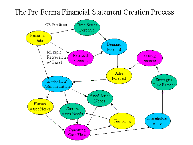
Pro forma financial statements are extremely vital decision-making tools for a firm’s managers and stakeholders. Managers use pro forma statements to forecast profits and financing needs at a given demand. Creditors often employ pro forma statements in predicting whether a firm will have the cash flow to service its debt. Finally, stockholders utilize pro forma statements to forecast a firm’s stock price or to value the equity of the firm.

Harley-Davidson, America’s leading motorcycle manufacturer, represents a fairly simple candidate for demand forecasting and pro forma financial statement determination, because Harley is not a diversified firm. Harley’s exit from the recreational vehicle market in 1995 made it essentially a one-product firm, and a large majority of its sales are domestic. The company’s motorcycle sales drive the demand for the firm’s tie-in products—parts, accessories, licensed apparel, and financing.

Demand Forecasting

The first step in determining the pro forma financial statement is to forecast sales, which drive most expenses and balance sheet accounts. Of course, sales are set in motion by demand for the product, so we must first forecast quantity demanded.

Since motorcycle sales are the key driver of Harley’s financial statements, our data consist of motorcycle units sold for 24 quarters beginning in 1996 and ending in 2001.

Year	Qtr	Units	Qtr	Units	Qtr	Units	Qtr	Units
1996	I	30,071	II	30,852	III	28,013	IV	29,835
1997	I	32,860	II	33,965	III	31,503	IV	33,957
1998	I	34,482	II	37,753	III	36,428	IV	42,155
1999	I	41,181	II	44,771	III	42,615	IV	48,620
2000	I	49,057	II	53,329	III	48,077	IV	54,129
2001	I	54,154	II	60,161	III	56,611	IV	63,535

The data are processed in the time-series forecasting program CB Predictor program, which is set to forecast the unit sales for the next four quarters. Demand is particularly strong in the second and fourth quarters, so directing CB Predictor to use seasonal forecasting techniques is critical. Therefore, the technique with the lowest root mean square error (RMSE) and mean absolute deviation (MAD) is not surprisingly the Holt-Winters’ multiplicative method. The forecast also yields higher unit sales in the second and fourth quarters relative to the other two quarters.

Methods	Rank	RMSE	MAD	MAPE
Double Exponential Smoothing	6	2617.1	2126.6	5.19
Double Moving Average	5	2442.9	1873.3	3.912
Holt-Winters' Additive	2	1664.9	1302.4	3.351
Holt-Winters' Multiplicative	1	1379.2	1283.4	3.21
Seasonal Additive	4	2423.9	2037	5.066
Seasonal Multiplicative	3	2319.3	1921.6	4.633
Single Exponential Smoothing	8	3410.7	2797.6	6.307
Single Moving Average	7	3291.5	2850.7	6.463

Time-series analysis provides only one piece of the forecasting puzzle. Several variables help to explain the variation in the residuals between the historical data for 24 quarters and the best time-series fit. In single-variable regression, the lagged percentage change in GDP explains 19.5% of the residuals’ variation; the 5-year Treasury rate explains 12.9%; and the inflation-adjusted Harley price explains 15.0%. The coefficient for the lagged GDP, however, is not intuitively correct, and this variable loses its significance in multivariate regression models. The best model for predicting the residual incorporates both the 5-year Treasury rate and the inflation-adjusted Harley price, and all variables are significant within a 90% level of confidence. It statistically explains only 27.1% of the variation in the residuals, but for a real-world model this is satisfactory.

Regression Statistics
Multiple R	0.521
R Square	0.271
Adjusted R Square	0.202
Standard Error	1257
Observations	24

ANOVA	df	SS	MS	F	Signif. F
Regression	2	12365073	6182537	3.911	0.036
Residual	21	33198016	1580858
Total	23	45563089
Variables	Coefficients	Standard Error	t Stat	P-value
Intercept	35066.66	17781.70	1.972	0.062
T-rates	-66415.74	35573.41	-1.867	0.076
Indexed Price	-3.139	1.81	-1.736	0.097

Year	Qtr	Time Ser	Modeled	Qtr	Time Ser	Modeled	Qtr	Time Ser	Modeled	Qtr	Time Ser	Modeled
		Residual	Residual		Residual	Residual		Residual	Residual		Residual	Residual
1996	I	1,540	360	II	-1,416	3	III	-1,308	-839	IV	-2,053	-1,001
1997	I	1,200	-478	II	1,240	715	III	-586	-891	IV	-1,551	-936
1998	I	-1,211	-84	II	439	-391	III	1,202	333	IV	1,682	477
1999	I	-2,142	487	II	371	806	III	1,067	116	IV	1,455	-491
2000	I	-772	-555	II	1,047	152	III	-1,061	164	IV	674	71
2001	I	-1,322	960	II	2,518	1,604	III	1,564	1,229	IV	1,382	1,099

The final step in the demand-planning model is to combine the results of the time-series model and the regression model to forecast future demand. CB predictor, using the Holt Winters’ Multiplicative method, modeled demand for the four quarters of 2002. For example, the trend and seasonal patterns of the historical data suggest that demand will be 64,761 motorcycles in the first quarter. We then adjust the time-series forecast using our multiple regression model. The low interest rates, interpolated from the forecasts of the GSU Economic Forecasting Center, will increase demand beyond the time-series forecast. Since the economy remains sluggish and Harley’s market share has eroded from 50% in 1997 to 45% in 2001, we expect inflation-adjusted prices to be low, especially in the first half of 2002. The combined effect of low prices and low interest rates gives Harley an adjusted demand of 66,205 motorcycles in the first quarter.

2002 Forecasts
	Time Ser	5-Year	CPI-index	Adjusted
Qtr	Output	T-Rate	Price	Output
I	64,761	4.3%	$ 9,800	66,205
II	68,356	4.6%	$ 9,800	69,600
III	62,817	4.8%	$ 9,900	63,615
IV	69,138	5.0%	$ 9,950	69,646

Historical Financial Statements

Harley-Davidson’s financial statements of the last six years give insight into the future direction of the company. Its profitability performance in the last six years has been outstanding, with profits and sales increasing every year. Sales have increased at an average annual rate of 17.0% during that period, which is remarkable growth for a manufacturer. More important, profits have increased at an average annual rate of 25.0%. The net profit margin has increased every year, from 9.4% in 1996 to 13.0% in 2001.

Most of the profit margin improvement in early years came from price increases that exceeded inflation. However, in 2001 gross margin increased from more efficient production and lower materials costs amid slightly lower motorcycle prices. By using Harley-Davidson Credit to finance an increasing number of its motorcycle sales, Harley has also improved its profit margins.

Harley’s advertising increased 7.0% to $203.1 million in 2001 and its R&D grew only 6.5% to $80.7 million in 2001 amid a 15.7% increase in sales. Since these expenditures are not increasing with sales, one must wonder whether the company is sacrificing market share and future sales for short-term profits.

Harley Income Statement and Common-Size Income Statement

	2001	2000	1999	1998	1997	1996
Net sales	3,363,414	2,906,365	2,452,939	2,063,956	1,762,569	1,531,227
Cost of goods sold	2,183,409	1,915,547	1,617,253	1,373,286	1,176,352	1,041,133
Gross profit	1,180,005	990,818	835,686	690,670	586,217	490,094
Selling, administrative and engineering expense	566,694	503,333	438,085	366,222	320,731	262,001
Motorcycle Income	613,311	487,485	397,601	324,448	265,486	228,093
Financial Svcs. Income	61,273	37,178	27,685	20,211	12,355	7,801
Corporate Expense	12,083	9,691	9,427	11,043	7,838	7,448
Income from Operations	662,501	514,972	415,859	333,616	270,003	228,446
Gain on sale of credit card business	0	18,915	0	0	0	0
Interest income, net	17,478	17,583	8,014	3,838	7,871	3,309
Other, net	6,524	2,914	3,080	-1,215	-1,572	-4,133
Income before provision for income taxes	673,455	548,556	420,793	336,229	276,302	227,622
Provision for income taxes	235,709	200,843	153,592	122,729	102,232	84,213
Net income	437,746	347,713	267,201	213,500	174,070	143,409

	2001	2000	1999	1998	1997	1996
Net sales	100.0%	100.0%	100.0%	100.0%	100.0%	100.0%
Cost of goods sold	64.9%	65.9%	65.9%	66.5%	66.7%	68.0%
Gross profit	35.1%	34.1%	34.1%	33.5%	33.3%	32.0%
Selling, administrative and engineering expense	16.8%	17.3%	17.9%	17.7%	18.2%	17.1%
Motorcycle Income	18.2%	16.8%	16.2%	15.7%	15.1%	14.9%
Financial Svcs. Income	1.8%	1.3%	1.1%	1.0%	0.7%	0.5%
Corporate Expense	0.4%	0.3%	0.4%	0.5%	0.4%	0.5%
Income from Operations	19.7%	17.7%	17.0%	16.2%	15.3%	14.9%
Gain on sale of credit card business	0.0%	0.7%	0.0%	0.0%	0.0%	0.0%
Interest income, net	0.5%	0.6%	0.3%	0.2%	0.4%	0.2%
Other, net	0.2%	0.1%	0.1%	-0.1%	-0.1%	-0.3%
Income before provision for income taxes	20.0%	18.9%	17.2%	16.3%	15.7%	14.9%
Provision for income taxes	7.0%	6.9%	6.3%	5.9%	5.8%	5.5%
Net income	13.0%	12.0%	10.9%	10.3%	9.9%	9.4%

Harley-Davidson has historically had a very conservative and well-managed balance sheet. The firm has maintained a debt-to-equity ratio of less than one, despite having a financing subsidiary that carries a lot of debt. Even without Harley-Davidson Credit, the company earned more interest income than interest expense, so it obviously preferred not to have much debt on the balance sheet. Obviously, most of Harley’s cash flow invested in fixed assets was generated by the company’s operations, not from borrowing.

Harley’s accounts receivable days have supposedly decreased. Harley-Davidson Credit is financing an increasing proportion of the company’s sales, so we would expect the A/R days to decline in line with an increase in finance receivables. The fixed asset turnover has remained stable, meaning that the company has invested in fixed assets at about the same rate as sales growth. The retirement liabilities have decreased as a percentage of sales, because Harley’s sales and profits grew at a much faster rate than its pension and other retirement liabilities. The firm’s accounts payable days have been virtually unchanged, and Harley’s inventory days were stable until a steady decline in 2001. In 2001 the motorcycle manufacturer must have slowed purchases in expectation of slower demand, although demand has remained steady.

Harley Balance Sheet and Balance Sheet Ratios

	2001	2000	1999	1998	1997	1996
ASSETS	(In thousands, except share amounts)
Current assets:
Cash and mkt. securities	635,449	419,736	183,415	165,170	147,462	142,479
Accounts receivable, net	118,843	98,311	101,708	113,417	102,797	141,315
Current portion of finance receivables, net	656,421	530,859	440,951	360,341	293,329	183,808
Inventories	181,115	191,931	168,616	155,616	117,475	101,386
Deferred income taxes	38,993	28,280	29,434	29,076	24,941	25,999
Prepaid expenses & other current assets	34,443	28,147	24,870	21,343	18,017	18,142
Total current assets	1,665,264	1,297,264	948,994	844,963	704,021	613,129

Finance receivables, net	379,335	234,091	354,888	319,427	249,346	154,264
Property, plant, and equipment, net	891,820	754,115	681,741	627,759	528,869	409,434
Goodwill, net	49,711	54,331	55,408	51,197	38,707	40,900
Other assets	132,365	96,603	71,046	76,863	77,958	82,258
	3,118,495	2,436,404	2,112,077	1,920,209	1,598,901	1,299,985

LIABILITIES AND SHAREHOLDERS’ EQUITY
Current liabilities:
Accounts payable	194,683	169,844	137,660	122,722	106,112	100,699
Accrued expenses and other liabilities	304,376	238,390	199,331	199,051	164,938	142,334
Current portion of finance debt	217,051	89,509	181,163	146,742	90,638	8,065
Total current liabilities	716,110	497,743	518,154	468,515	361,688	251,098

Finance debt	380,000	355,000	280,000	280,000	280,000	250,000
Other long-term liabilities	176,190	97,340	77,124	69,700	62,131	70,366
Postretirement health care benefits	89,912	80,666	75,719	72,083	68,414	65,801
Shareholders’ equity:
Common Stock	3,242	3,210	1,592	1,584	1,572	1,562
Additional paid-in capital	359,165	285,390	236,540	211,960	187,180	174,371
Retained earnings	1,833,335	1,431,017	1,113,376	873,171	683,824	530,782
Accumulated other comprehensive income	-13,728	308	-2,067	1,128	-2,835	-566
	2,182,014	1,719,925	1,349,441	1,087,843	869,741	706,149
Less: Treasury stock	-425,546	-313,994	-187,992	-57,133	-41,959	-41,933
Unearned compensation	-185	-276	-369	-799	-1,114	-1,496
Total shareholders’ equity	1,756,283	1,405,655	1,161,080	1,029,911	826,668	662,720
	3,118,495	2,436,404	2,112,077	1,920,209	1,598,901	1,299,985

	2001	2000	1999	1998	1997	1996

Inventory Days	30	37	38	41	36	36
A/R Days	13	12	15	20	21	34
Current Fin. Receivables/Sales	19.5%	18.3%	18.0%	17.5%	16.6%	12.0%
Deferred Taxes/Pretax Income	5.8%	5.2%	7.0%	8.6%	9.0%	11.4%
Prepaid Expenses/Sales	1.0%	1.0%	1.0%	1.0%	1.0%	1.2%
Long-term Fin. Receivables/Sales	11.3%	8.1%	14.5%	15.5%	14.1%	10.1%
Fixed Asset Turnover	3.8	3.9	3.6	3.3	3.3	3.7
Other Assets/Sales	3.9%	3.3%	2.9%	3.7%	4.4%	5.4%
A/P Days	33	32	31	33	33	35
Accrued Expenses/Sales	9.0%	8.2%	8.1%	9.6%	9.4%	9.3%
Other Long-term Liab./Sales	5.2%	3.3%	3.1%	3.4%	3.5%	4.6%
Retirement Benefits/Sales	2.7%	2.8%	3.1%	3.5%	3.9%	4.3%

Risk Factors

Before we can create Harley-Davidson’s forecasted financial statements, we must understand the firm’s risk factors. One risk factor is that Harley’s average customer is getting older. For example, the average Harley buyer in the mid-1980’s was in his mid-30’s, and today the average buyer is in his mid-40’s. Harley will probably have to increase advertising and product development to appeal to younger motorcycle buyers, but without alienating its core market group.

Another risk factor is that Harley’s Japanese competitors will continue to increase market share in the heavyweight motorcycle market amid Harley’s inability to satisfy firm demand. The American company will have to continue to invest in new capacity, and it will probably have to increase advertising and keep prices low in order to improve market share.

Other risk factors include potential environmental regulations, the chance of a strike (despite healthy relations with its union), foreign exchange risk, and a cyclical business trend. Because Harley-Davidson motorcycles are largely recreational products, we would have expected sales to suffer in late 2001 as the economy slowed; however, demand has remained strong.

Pro Forma Financial Statements

Using our demand model, our historical financial statements and ratios, and our risk factors, we will generate our expected pro forma statements. Then we will apply Monte Carlo simulation to determine the variability to several financial accounts, like net income and borrowing, given the probability distributions of a few critical environmental and firm variables.

The first and most crucial part of creating pro forma statements is to forecast sales. The demand model predicted an adjusted total demand of 269,066 motorcycles in 2002. Because of competitive and environmental stresses, we expect that the price per motorcycle will be fairly low, between $9,800 and $9,900 in first quarter 1996 dollars. Using the GSU Economic Forecasting Center’s CPI predictions for 2002, the average motorcycle price will be $11,374; hence, the total motorcycle revenue will be $3.06 billion. Since Harley-Davidson motorcycles have constituted between 77% and 78.5% of revenues from 1996 to 2001, we will assume they make up 77.75% of revenues. Therefore, the total sales for the whole company will be $3.95 billion, a 14.8% increase over 2001.

The gross profit margin will decrease to 33.5% in 2002 because of the slow economy and Harley’s desire to improve market share. This decline will be partially offset by decreases in the cost of metals and other raw materials. Harley-Davidson’s general and administrative expenses will increase to 17.5% of sales as the motorcycle manufacturer spends more on advertising and develops new products for younger customers. The company’s corporate expenses and interest income will stay constant, as a percent of sales; and its financial services income will increase to 2.0% of sales, as the division benefits from the low interest rate environment.

The balance sheet accounts are more difficult to forecast, because many of the accounts, especially the long-term assets and liabilities, do not vary with sales. However, forecasting the balance sheet is critical to any investor or banker, because it indicates how much the firm is borrowing and where the firm is investing its funds. In Harley’s case, we assume that the balance sheet accounts will follow the trends of the last six years or they, in the case of inventory, revert to the mean of the last several years.

Assumptions		2002

Gross Profit Margin		33.5%
General and Admin/Sales		17.5%
Corporate Expenses/Sales		0.4%
Interest Income (Net)/Sales		0.5%
Financial Svcs Income/Sales		2.0%
Income Tax Rate		36.0%
Inventory Days		35
A/R Days		12
Current Fin. Receivables/Sales		20.5%
Deferred Taxes/Pretax Income		5.5%
Prepaid Expenses/Sales		1.0%
Long-term Fin. Receivables/Sales		10.0%
Fixed Asset Turnover		3.8
Other Assets/Sales		3.5%
A/P Days		33
Accrued Expenses/Sales		9.0%
Other Long-term Liab./Sales		4.0%
Retirement Benefits/Sales		2.5%
Dividends/Net Income		10.0%
Cash/Sales		10.0%

Pro Forma Income Statement	2002

Sales	3,949,015
Cost of Goods Sold	2,626,095
Gross Profit	1,322,920
General & Admin Expenses	691,078
Motorcycle Income	631,842
Financial Svcs. Income	78,980
Corporate Expense	15,796
Income from Operations	695,027
Interest Income (Net)	19,745
Income before Taxes	714,772
Provision for Income Taxes	257,318
Net Income	457,454

Pro Forma Balance Sheet		Dec. 31, 2002

Cash and Marketable Securities	394,902	Accounts Payable	237,428
Accounts Receivable, Net	129,831	Accrued Expenses	355,411
Current Portion of Fin. Receivables	809,548	Current Portion of Finance Debt	-
Inventories	251,817	Total Current Liabilities	592,839
Deferred Income Taxes	39,312	Finance Debt	380,000
Prepaid Expenses	39,490	Other Long-term Liabilities	157,961
Total Current Assets	1,664,900	Postretirement health care benefits	98,725
Finance Receivables, Net	394,902	Common Stock	3,242
Property, Plant, & Equipment, Net	1,039,215	Additional Paid-in Capital	359,165
Goodwill, Net	45,000	Retained Earnings	2,245,044
Other Assets	138,216	Treasury Stock	(554,744)
Total Assets	3,282,232	Total Liabilities & Equity	3,282,232

To create the pro forma statements, the analyst merely adheres to the assumptions inherent in trend and risk analysis. First we construct the income statement, and knowing the estimated net income and dividends, we can determine the change in retained earnings. Once we have the change in retained earnings and we have estimated fixed asset and working capital investments, we generate the pro forma balance sheets. We assume no stock issuances or long-term debt issuances, and we finally calculate Harley-Davidson’s financing shortfall, if any. Since Harley-Davidson had abundant cash flow from operations, it has a cash surplus of $346 million.

From here we must determine the optimal use of that surplus cash and how it affects the balance sheet. Of course, the firm could increase its dividend, but buying back stock (that is, treasury stock) has been Harley’s preferred means of distributing funds to investors. Harley could also pay off its short-term debt in order to reduce the already low borrowing costs of Harley-Davidson Credit. We will assume that long-term debt cannot be prematurely liquidated. If reimbursing its short-term debtors takes precedence over buying back stock, Harley will pay back all its short-term debt and will purchase $129 million of its shares.

The pro forma statements could be complicated by our changes. By purchasing its shares, Harley is saving cash on dividend payments, and it is also saving interest by decreasing its borrowing. The lower interest expenses, for example, will increase Harley-Davidson’s profits, increase retained earnings, and enable the firm to borrow even less, therefore saving more on interest. We could easily develop an optimization model that runs this iteration numerous times and solves for pro forma statements to the penny.* For our purposes, we will assume that the interest savings from less debt will exactly offset the interest loss from having lower cash balances and short-term investments.

*Interest income or expense would equal the ending total debt balance times an interest rate. Changes in interest income or interest income would feed into net income and hence retained earnings. The optimization model would minimize short-term debt and minimize treasury stock (a negative number), with the constraints that total assets must equal total liabilities and equity, that short-term debt must be at least zero, and that treasury stock could not increase. (In the real world, borrowing in order to purchase treasury stock may be feasible, but it will not occur in this model, even if we incorporate Harley’s low dividend rate into the model.)

Page 2—Pro Form Scenarios and Simulation

Pro Forma Financial Statement Determination: Harley-Davidson

Introduction

Demand Forecasting

Units

Units

Units

Units

Variables

Historical Financial Statements

Pro Forma Financial Statements